Project 12 · Part VII: Projects
Visualizing and Attacking a CNN
Open up the CIFAR-10 network of Project 9: see which pixels and regions drive its decisions with saliency maps and Grad-CAM, break it with imperceptible adversarial perturbations, and partly repair it with adversarial training.
After this project you will be able to
- Compute gradient saliency maps and Grad-CAM heat maps for a trained CNN.
- Implement FGSM and PGD attacks with an $\ell_\infty$ budget in pixel units, and plot accuracy against the budget.
- Fine-tune a network on adversarial examples and measure the trade-off between robustness and clean accuracy.
Code: projects/p12_vis_attack/ (vis_attack.py, tests/). It uses the network trained in Project 9. Background: Chapters 22 and 17.
P12.1The Problem
The CNN of Project 9 classifies 86% of the CIFAR-10 test images correctly. This project asks two questions about it. What does it look at when it makes a decision? And how robust is that decision to small, deliberately chosen changes of the input? The first is answered with the attribution methods of Section 22.2, the second with the attacks and defenses of Section 22.4.
P12.2The Data
We use the first 1,000 CIFAR-10 test images for evaluation and, for adversarial fine-tuning, 10,000 randomly chosen training images. All attacks work with pixel values in $[0,1]$, so that the perturbation budget $\varepsilon$ has a direct meaning: $\varepsilon=4/255$ means that no color value of any pixel changes by more than 4 of its 256 possible levels, a change too small to see. A small wrapper module applies the channel normalization of Project 9 inside the model, so the attack code never needs to know about it.
P12.3Building It from Scratch
Saliency and Grad-CAM. The saliency map is one backward pass: the gradient of the predicted class’s score with respect to the input pixels, maximized over color channels (Equation (22.1)). Grad-CAM (Equation (22.3)) uses the $8\times8$ feature maps of the last convolutional block, captured with a forward hook, weights each channel by the spatial average of the gradient of the class score with respect to it, keeps the positive part of the weighted sum, and upsamples the result to the image size:
import torch
import torch.nn.functional as F

def grad_cam(model, x, cls):
    """Eq. (22.3) on the last convolutional block (8x8 maps), upsampled to the image size."""
    feats = {}
    h = model.model.features.register_forward_hook(lambda m, i, o: feats.__setitem__("A", o))
    scores = model(x)
    h.remove()
    A = feats["A"]
    grads = torch.autograd.grad(scores[torch.arange(len(x)), cls].sum(), A)[0]
    weights = grads.mean((2, 3), keepdim=True)                          # alpha_k: averaged gradients
    cam = F.relu((weights * A).sum(1, keepdim=True))
    cam = F.interpolate(cam, size=x.shape[-2:], mode="bilinear", align_corners=False)[:, 0]
    return cam / (cam.amax((1, 2), keepdim=True) + 1e-8)
Attacks. FGSM takes one step of size $\varepsilon$ in the direction of the sign of the loss gradient (Equation (22.5)). PGD starts from a random point in the $\varepsilon$-ball, takes 10 signed steps of size $2.5\varepsilon/10$, and after each step projects back onto the ball and the valid pixel range (Equation (22.6)). Both evaluate the model in evaluation mode, so that batch normalization uses its running statistics and the attack sees the same function that is deployed.
Adversarial fine-tuning. Starting from the trained network, we run one pass over 10,000 training images in batches of 128, replacing every batch by PGD adversarial examples (3 steps, $\varepsilon=4/255$, generated with the current weights) and taking an SGD step on them (Equation (22.7)). This is a short and cheap version of adversarial training; full adversarial training runs PGD on every batch for the whole training run, which multiplies its cost by the number of attack steps.
P12.4Using Libraries
Everything here is a few lines of PyTorch around torch.autograd. Libraries such as Captum provide saliency, integrated gradients, Grad-CAM, and many other attribution methods for arbitrary models, and adversarial-robustness libraries provide attacks, including strong adaptive ones, together with evaluation protocols. Before trusting a claimed defense, evaluate it with such standardized attack suites rather than with your own attacks alone (Chapter 22).
P12.5Results and Discussion
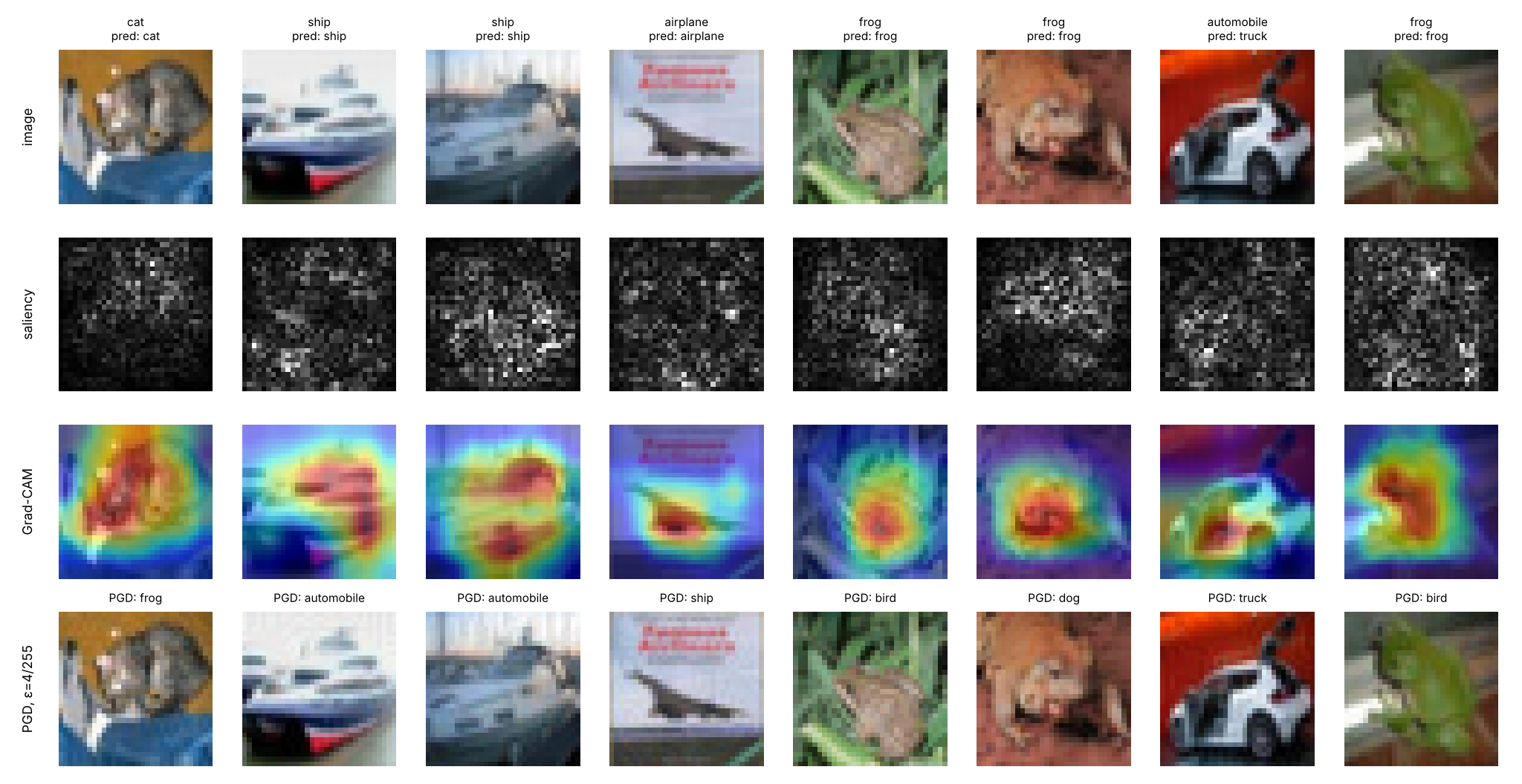
Attribution. The saliency maps are speckled: individual pixel gradients are noisy, though brighter on the objects than on the background. Grad-CAM maps are coarse but clearly object-centered: on the cat, the frogs, and the ships the heat covers the animal or the hull, and on the airplane the plane rather than the text above it. Note that a heat map shows where the evidence for the predicted class lies, not that the prediction is right: the automobile misclassified as a truck gets a confident heat map on the car’s body. Grad-CAM’s coarseness is a consequence of its $8\times8$ feature maps; the method trades resolution for class-specific, less noisy maps.
Attacks. Accuracy on the first 1,000 test images against the $\ell_\infty$ budget:
| $\varepsilon\times255$ | 0 | 1 | 2 | 4 | 8 |
|---|---|---|---|---|---|
| FGSM, trained network | 87.6% | 49.9% | 28.4% | 9.3% | 4.6% |
| PGD, trained network | 87.6% | 43.0% | 10.0% | 0.1% | 0.0% |
| PGD, after adversarial fine-tuning | 66.8% | 58.8% | 50.1% | 36.3% | 13.2% |
A perturbation of a single intensity level per pixel ($\varepsilon=1/255$) halves the network’s accuracy, and four levels, invisible in Figure P12.1, reduce it to essentially zero under PGD. PGD is consistently stronger than FGSM because it can follow the curvature of the loss rather than trusting its linearization; FGSM’s accuracy even stops falling at large $\varepsilon$, a sign that a single step overshoots. The predictions of the adversarial images in the figure are not random: ships become automobiles and frogs become birds or dogs, classes that are already nearby in the network’s feature space.
Defense and its cost. One pass of adversarial fine-tuning over 10,000 images, about a minute and a half of computation, raises the accuracy under PGD at $\varepsilon=4/255$ from 0.1% to 36%, and to 13% even at twice the budget it was trained for. But clean accuracy falls from 87.6% to 66.8%. Part of that drop would be recovered by longer adversarial training from scratch, but a gap between clean and robust accuracy persists in the best known models: robustness to $\ell_\infty$ perturbations requires features that ignore small, high-frequency patterns that are genuinely useful for clean accuracy.
P12.6Extensions
- Implement integrated gradients (Equation (22.2)) with a black baseline and 50 steps, check completeness numerically, and compare the maps with plain saliency.
- Run the sanity check of Adebayo et al. (2018): randomize the weights of the last block and recompute the Grad-CAM maps. Do they change as they should?
- Make the attacks targeted: turn every test image into a “frog.” How large must $\varepsilon$ be to succeed on 90% of images?
- Test transferability: craft PGD examples against a second CNN trained with a different random seed and evaluate them on the original network.
- Run full adversarial training for 10 epochs and plot clean and robust accuracy over training.